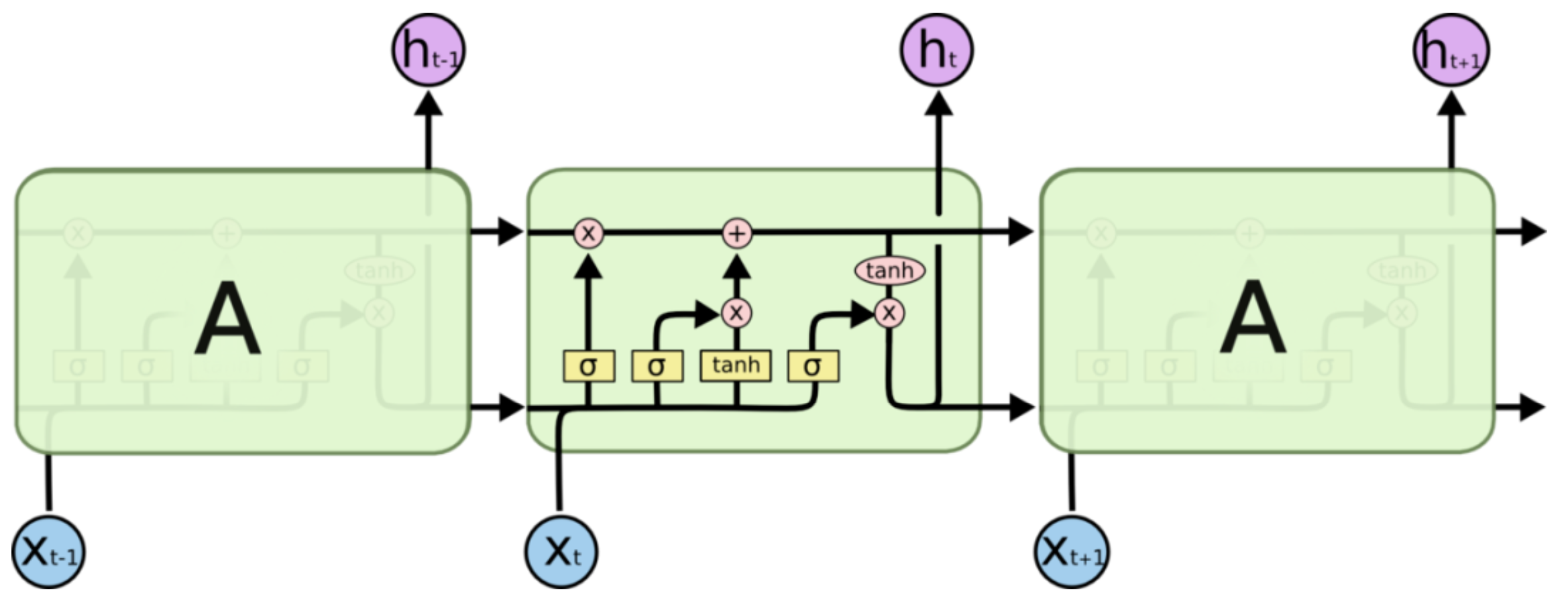
LSTM (Long Short-Term Memory) 长短期记忆网络

1.网络神经元结构

$$NDVI=\frac{NIR近红外-RED红色}{NIR近红外+RED红色}$$

遗忘门 (forget gate)：$f_t=\sigma(W_f\cdot[x_t,h_{t-1}]+b_f)$ 表示对信息的记忆程度；
输入门 (input gate)：$i_t=\sigma(W_i\cdot[x_t,h_{t-1}]+b_i)$ ，表示对信息的输入强度；
状态门 (cell gate)：$g_t=tanh(W_g\cdot[x_t,h_{t-1}]+b_g)$ ，表示对输入信息的处理；
输出门 (output gate)：$o_t=\sigma(W_o\cdot[x_t,h_{t-1}]+b_o)$ ，表示对信息的输出强度；

其中，$[x_t,h_{t-1}]$ 表示两向量的并列 (concatenate) 向量，$ht_{t-1}$表示神经元 t-1 时刻的隐藏状态，$\sigma$ 为 sigmoid 函数。

在此基础上可更新神经元 � 时刻的细胞状态 �� 与隐藏状态 ℎ� 如下：

��=��⊙��−1+��⊙��，即细胞状态 = 经过遗忘后的旧细胞状态 + 神经元处理后的新信息；
ℎ�=��⊙tanh⁡(��)，即隐藏状态 = 输出强度 × tanh处理后的细胞状态；

其中 ⊙ 表示哈达玛积 (Hadamard product)，即向量对应元素相乘。

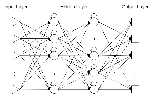
2.多层LSTM 网络结构

3.构建LSTM 网络

声明数据

声明网络

LSTM数据格式：

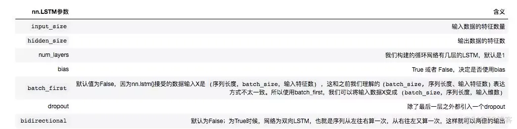
num_layers: 我们构建的循环网络有层lstmnum_directions: 当bidirectional=True时，num_directions=2；当bidirectional=False时，num_directions=1

输入LSTM中的数据格式

输入LSTM中的X数据格式尺寸为(seq_len, batch, input_size)，此外h0和c0尺寸如下
h0(num_layers * num_directions, batch_size, hidden_size)
c0(num_layers * num_directions, batch_size, hidden_size)

LSTM输出数据格式

LSTM输出的数据格式尺寸为(seq_len, batch, hidden_size * num_directions)；输出的hn和cn尺寸如下hn(num_layers * num_directions, batch_size, hidden_size)
cn(num_layers * num_directions, batch_size, hidden_size)

#x: 这里我们将x的尺寸 (batch_size, seq_len, dims)依次是(3, 5, 4)
x = t.randn(3, 5, 4) 
x
tensor([[[ 0.1478, -0.7733, -0.3462,  0.0320],
         [-0.0540,  0.4757, -1.2787,  0.6141],
         [ 1.9581,  0.0015,  1.4387, -0.5895],
         [-1.0691, -1.7070,  1.0219, -0.7990],
         [-1.7735,  0.6824,  0.6067, -0.6630]],

        [[-0.3223, -0.6943,  0.1120, -1.7799],
         [-1.0542,  0.2151, -2.2530,  0.2640],
         [-0.0599, -0.1996,  0.9793, -1.4952],
         [-0.2328,  0.2297, -1.4825,  0.0720],
         [ 0.7112, -0.1165,  2.5641, -1.4247]],

        [[-0.4157, -1.1617, -0.7442, -0.8369],
         [ 0.5266,  2.3119,  0.6428,  0.3797],
         [-0.2951, -1.5711,  1.2832, -0.2773],
         [ 0.4760,  0.2403,  0.2923,  2.2315],
         [-0.3348, -0.0976,  0.0388,  0.5948]]])